Modeling and Simulation Approaches
to Challenges in Nuclear Energy
Kathryn Huff
Rensselaer Polytechnic Institute
September 21, 2015


Insights at Disparate Scales


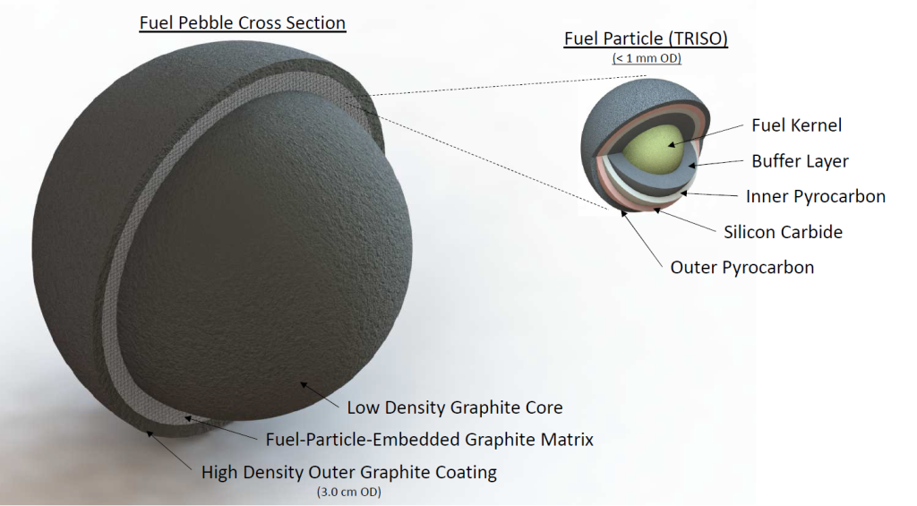
PB-FHR Fuel Geometry
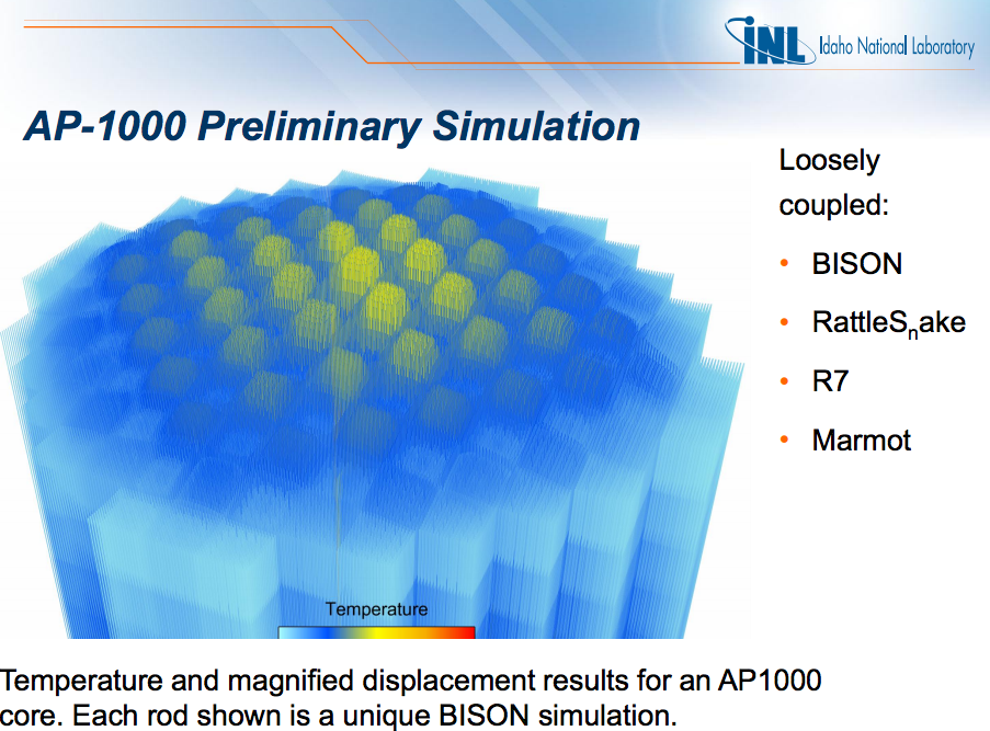
Coupled Multi-Physics Analysis
Severe accident neutronics and thermal hydraulics can be simulated beautifully for simple geometries and well studied materials. (below, INL BISON work.)
FHR, Accident Transient Analysis
- Collect experimental data
- Conduct algebraic, static, and benchmark results
- Develop 0D coupled neutronics/TH model (PyRK)
- Develop 3D neutronics/TH model
- Compare 0D and 3D models
- Connect additional coupled physics
PyRK: Python for Reactor Kinetics
Review of Nuclear Reactor Kinetics

\[\sigma(E,\vec{r},\hat{\Omega},T,x,i)\]

\[k=1\]
Reactivity
\[ \begin{align} k &= \mbox{"neutron multiplication factor"}\\ &= \frac{\mbox{neutrons causing fission}}{\mbox{neutrons produced by fission}}\\ \rho &= \frac{k-1}{k}\\ \rho &= \mbox{reactivity}\\ \end{align} \]Reactivity
\[ \rho(t) = \rho_0 + \rho_f(t) + \rho_{ext} \]where
\[ \begin{align} \rho(t) &= \mbox{total reactivity}\\ \rho_f(t) &= \mbox{reactivity from feedback}\\ \rho_f(t) &= \sum_i \alpha_i\delta T_i\\ T_i &= \mbox{temperature of component i}\\ \alpha_i &= \mbox{temperature reactivity coefficient of i}\\ \rho_{ext}(t) &= \mbox{external reactivity insertion}. \end{align} \]


\[\beta_i, \lambda_{d,i}\]
PyRK
- 6-precursor-group,
- 11-decay-group Point Reactor Kinetics model
- Lumped Parameter thermal hydraulics model
- Object-oriented, geometry and material agnostic framework
Point Reactor Kinetics
\[ \begin{align} p &= \mbox{ reactor power }\\ \rho(t,&T_{fuel},T_{cool},T_{mod}, T_{refl}) = \mbox{ reactivity}\\ \beta &= \mbox{ fraction of neutrons that are delayed}\\ \beta_j &= \mbox{ fraction of delayed neutrons from precursor group j}\\ \zeta_j &= \mbox{ concentration of precursors of group j}\\ \lambda_{d,j} &= \mbox{ decay constant of precursor group j}\\ \Lambda &= \mbox{ mean generation time }\\ \omega_k &= \mbox{ decay heat from FP group k}\\ \kappa_k &= \mbox{ heat per fission for decay FP group k}\\ \lambda_{FP,k} &= \mbox{ decay constant for decay FP group k}\\ T_i &= \mbox{ temperature of component i} \end{align} \]Lumped Parameter Heat Transfer
The heat flow out of body $i$ is the sum of surface heat flow by conduction, convection, radiation, and other mechanisms to each adjacent body, $j$: \[ \begin{align} Q &= Q_i + \sum_j Q_{ij}\\ &=Q_i + \sum_j\frac{T_{i} - T_{j}}{R_{th,ij}}\\ \dot{Q} &= \mbox{total heat flow out of body i }[J\cdot s^{-1}]\\ Q_i &= \mbox{other heat transfer, a constant }[J\cdot s^{-1}]\\ T_i &= \mbox{temperature of body i }[K]\\ T_j &= \mbox{temperature of body j }[K]\\ j &= \mbox{adjacent bodies }[-]\\ R_{th} &= \mbox{thermal resistence of the component }[K \cdot s \cdot J^{-1}]. \end{align} \]Quality Control
- Unit Checking: Pint (github.com/pint)
- Version Control: Git & GitHub (github.com/pyrk/pyrk)
- Automated Documentation: Sphinx (pyrk.github.io)
- Test Suite: nose
- Continuous Integration: Travis (travis-ci.org/pyrk/pyrk)
- Plotting: Matplotlib
- ODE solvers: SciPy
Unit Checking

In PyRK, the Pint package (pint.readthedocs.org/en/0.6/) is used keeping track of units, converting between them, and throwing errors when unit conversions are not sane.
Version Control

Keeping track of versions of the code makes it possible to experiment without fear and placing the code online encourages use and collaboration.
Automated Documentation

Automated documentation creates a browsable website explaining the most recent version of the code.
Test Suite

The classes and functions that make up the code are tested individually for robustness using nose.
Continuous Integration

The tests are run every time a change is made to the repository online. The results are public. If a main branch has a failed test, I get an email.
Neutronics : Reactivity Insertion Model

The reactivity insertion that drives the simulator can be selected and customized from three models.
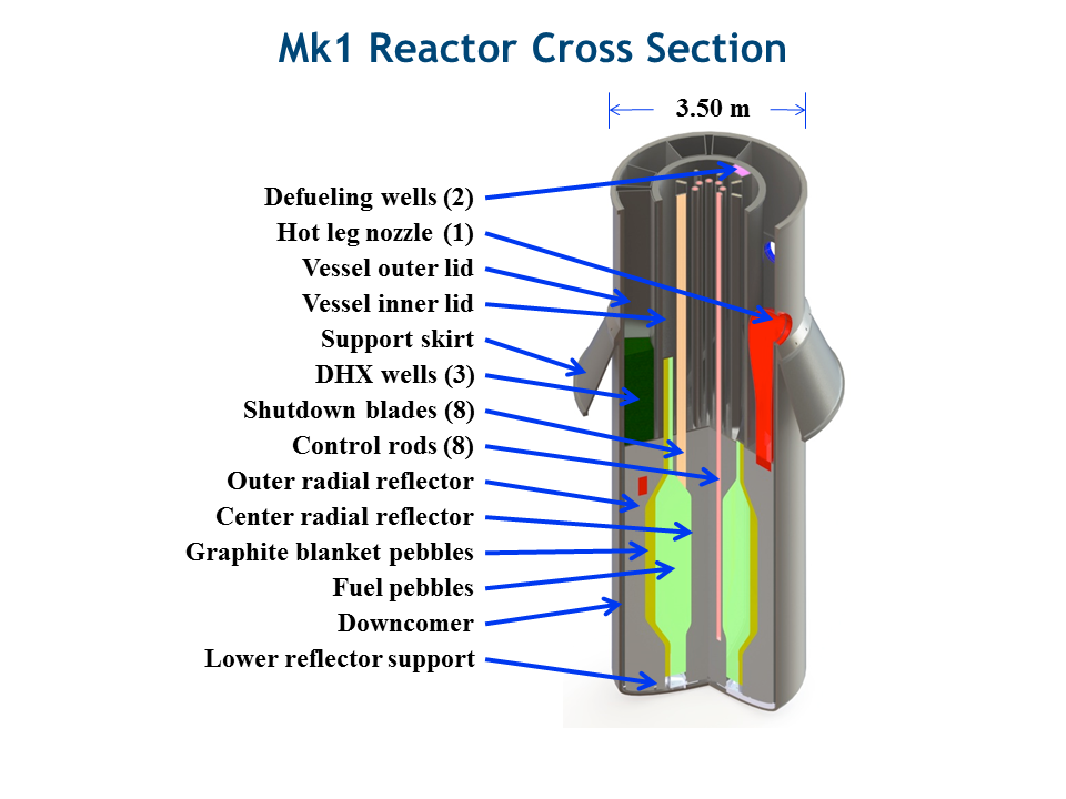
PB-FHR Reactivity Insertion
Pebble-Bed, Fluoride Salt Cooled, High-Temperature Reactor
- Molten FLiBe Coolant
- Annular Core
- Annular Pebble Fuel
- Steady Inlet Temperature
- Ramp Reactivity Insertion, 600pcm over 10s
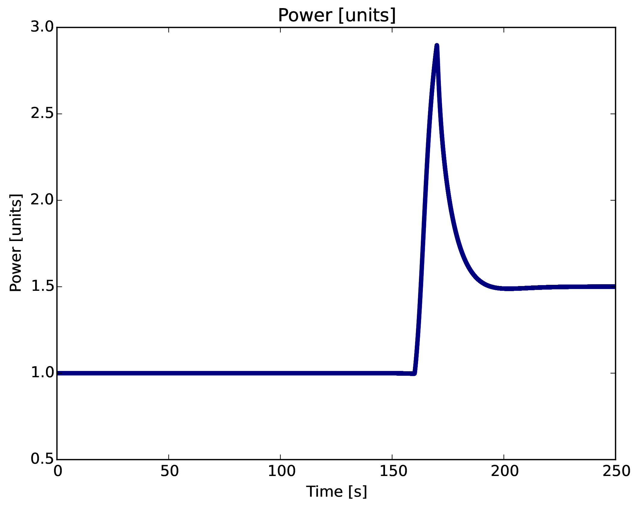
Ramp Reactivity Insertion

Ramp Reactivity Insertion
# External Reactivity
from reactivity_insertion import RampReactivityInsertion
rho_ext = RampReactivityInsertion(timer=ti,
                                  t_start=t_feedback + 10.0*units.seconds,
                                  t_end=t_feedback + 20.0*units.seconds,
                                  rho_init=0.0*units.delta_k,
                                  rho_rise=600.0*units.pcm,
                                  rho_final=600.0*units.pcm)
Impulse Reactivity Insertion
Components
fuel = th.THComponent(name="fuel",
                      mat=Fuel,
                      vol=vol_fuel,
                      T0=t_fuel,
                      alpha_temp=alpha_fuel,
                      timer=ti,
                      heatgen=True,
                      power_tot=power_tot/n_pebbles,
                      sph=True,
                      ri=r_mod,
                      ro=r_fuel
                      )

mod = th.THComponent(name="mod",
                     mat=Moderator,
                     vol=vol_mod,
                     T0=t_mod,
                     alpha_temp=alpha_mod,
                     timer=ti,
                     sph=True,
                     ri=0.0,
                     ro=r_mod)

cool = th.THComponent(name="cool",
                      mat=cool,
                      vol=vol_cool,
                      T0=t_cool,
                      alpha_temp=alpha_cool,
                      timer=ti)

shell = th.THComponent(name="shell",
                       mat=Shell,
                       vol=vol_shell,
                       T0=t_shell,
                       alpha_temp=alpha_shell,
                       timer=ti,
                       sph=True,
                       ri=r_fuel,
                       ro=r_shell)
Heat Transfer
# The coolant convects to the pebbles
cool.add_convection('pebble', h=h_cool, area=a_pb)
cool.add_advection('cool', m_flow/n_pebbles, t_inlet, cp=cool.cp)
Pebble Temperature
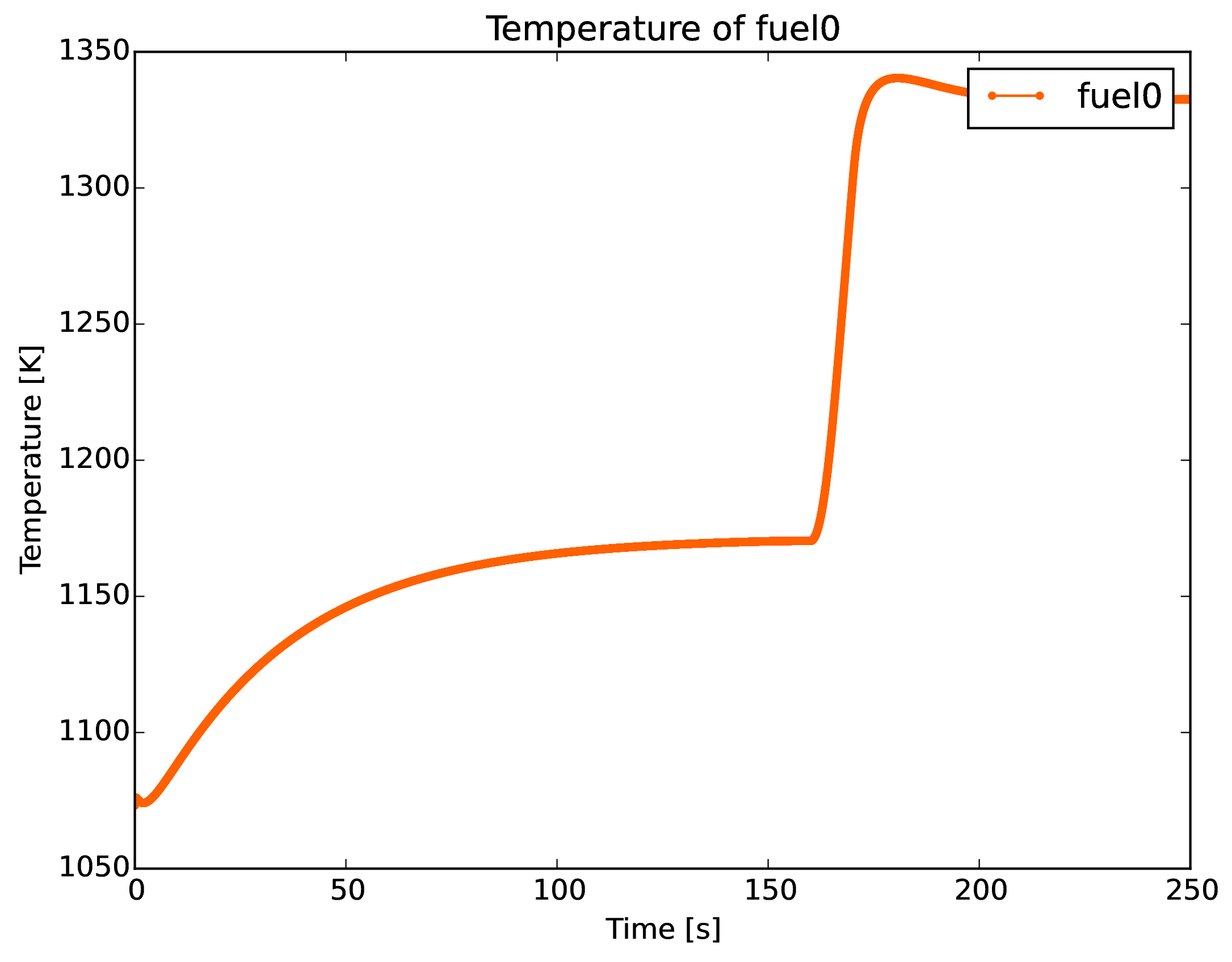
Average fuel pebble peak temperature \[<1100^\circ C\]
A Nuclear Fuel Cycle Simulation Framework
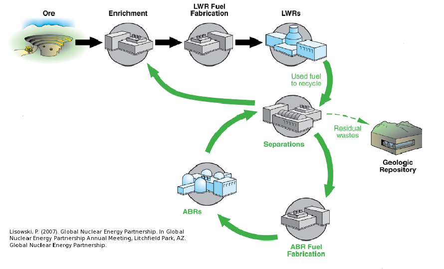
The Nuclear Fuel Cycle
Hundreds of discrete facilities mine, mill, convert, fabricate, transmute, recycle, and store nuclear material.
Fuel Cycle Metrics
- Mass Flow
- inventories, decay heat, radiotoxicity,
- proliferation resistance and physical protection (PRPP) indices.
- Cost
- levelized cost of electricity,
- facility life cycle costs.
- Economics
- power production, facility deployments,
- dynamic pricing and feedback.
- Disruptions
- reliability, safety,
- system robustness.
Current Simulators
- CAFCA (MIT)
- COSI (CEA)
- DANESS (ANL)
- DESAE (Rosatom)
- Evolcode (CIEMAT)
- FAMILY (IAEA)
- GENIUSv1 (INL)
- GENIUS v2 (UW)
- NFCSim (LANL)
- NFCSS (IAEA)
- NUWASTE (NWTRB)
- ORION (NNL)
- MARKAL (BNL)
- VISION (INL)
State of the Art
Performance
- Speed interactive time scales
- Fidelity: detail commensurate with existing challenges
- Detail: discrete material and agent tracking
- Regional Modeling: enabling international socio-economics
Beyond the State of the Art
Access
- Openness: for collaboration, validation, and code sustainability.
- Usability: for a wide range of user sophistication
Extensibility
- Modularity: core infrastructure independent of proprietary or sensitive data and models
- Flexibility with a focus on robustness for myriad potential developer extensions.
Extensibility

Openness
...Well Beyond
Algorithmic Sophistication
- Efficient: memory-efficient isotope tracking
- Customizable: constrained fuel supply
- Dynamic: isotopic-quality-based resource routing
- Physics-based: fuel fungibility
Agent Based Systems Analysis
An agent-based simulation is made up of actors and communications between those actors.
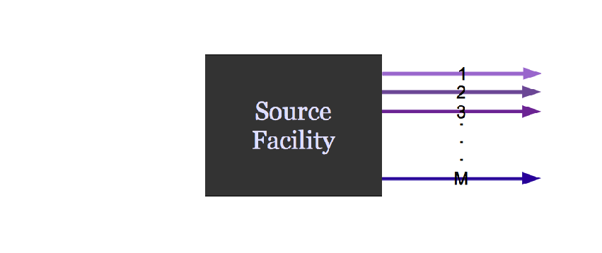
Agent Based Systems Analysis
A facility might create material.
Agent Based Systems Analysis
It might request material.
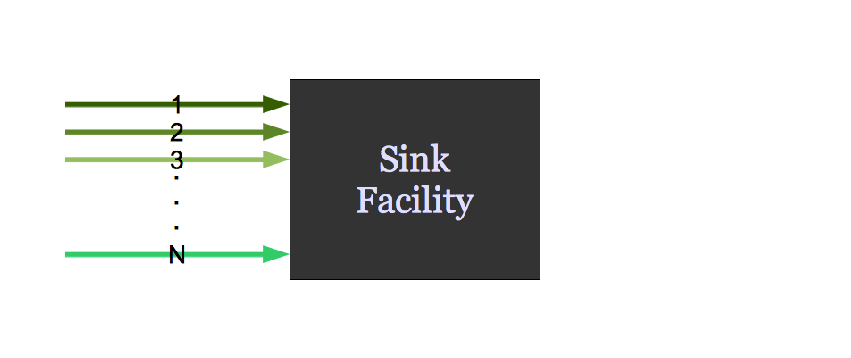
Agent Based Systems Analysis
It might do both.
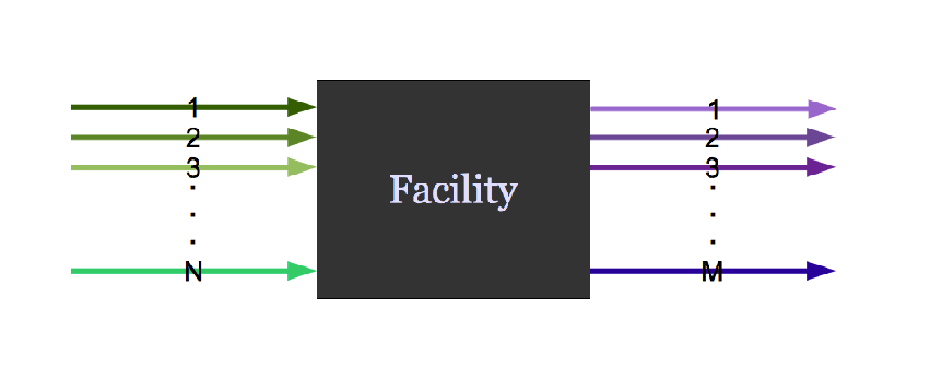
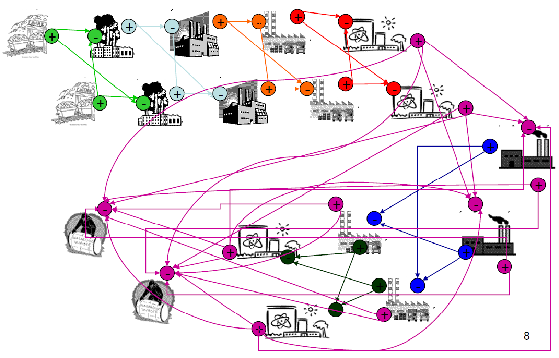
Agent Based Systems Analysis
Even simple fuel cycles have many independent agents.
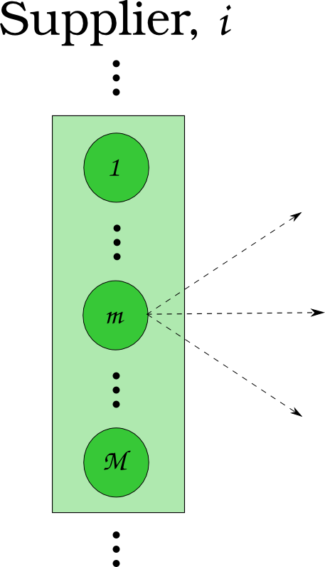
Agent Based Systems Analysis
 \[N_i \subset N\]
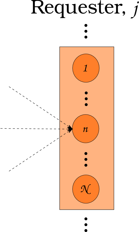
Agent Based Systems Analysis
 \[N_j \subset N\]
Agent Based Systems Analysis
 \[N_i \cup N_j = N\]
Feasibility vs. Optimization

If a decision problem is in NP-C, then the corresponding optimization problem is NP-hard.
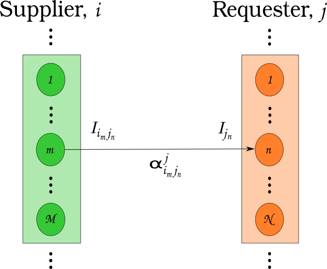
Transportation Formulation


Transportation Formulation
\[ \begin{align} \min_{x} z &= \sum_{i\in I}\sum_{j\in J} c_{i,j}x_{i,j} & \\ s.t & \sum_{i\in I_s}\sum_{j\in J} a_{i,j}^k x_{i,j} \le b_s^k & \forall k\in K_s, \forall s\in S\\ & \sum_{J\in J_r}\sum_{i\in I} a_{i,j}^k x_{i,j} \le b_r^k & \forall k\in K_r, \forall r\in R\\ & x_{i,j} \in [0,x_j & \forall i\in I, \forall j\in J \end{align} \]
Growing Ecosystem
Insights at Disparate Scales
Detailed Metrics

Material Attractiveness

Insights at Disparate Scales

Links
Acknowledgements
- Matthew Gidden
- Anthony Scopatz
- Massimiliano Fratoni
- Ehud Greenspan
- Per Peterson
- Xin Wang
- Paul Wilson
- Jasmina Vujic

THE END
Katy Huff
katyhuff.github.io/2015-09-21-rpi
Modeling and Simulation Approaches to Challenges in Nuclear Energy by Kathryn Huff is licensed under a Creative Commons Attribution 4.0 International License.
Based on a work at http://katyhuff.github.io/2015-09-21-rpi.